“ NLP - SENTIMENT ANALYSIS ON IMDB MOVIE DATASET ”
Use NLP for performing Sentiment Analysis

To make best out of this blog post Series , feel free to explore the first Part of this Series in the following order:-
- Dog Vs Cat Image Classification
- Dog Breed Image Classification
- Multi-label Image Classification
- Time Series Analysis using Neural Network
- NLP- Sentiment Analysis on IMDB Movie Dataset
- Basic of Movie Recommendation System
- Collaborative Filtering from Scratch
- Collaborative Filtering using Neural Network
- Writing Philosophy like Nietzsche
- Performance of Different Neural Network on Cifar-10 dataset
- ML Model to detect the biggest object in an image Part-1
- ML Model to detect the biggest object in an image Part-2
Before we start , I would like to thank Jeremy Howard and Rachel Thomas for their efforts to democratize AI. Thanks to the awesome fast.ai community for all the quick help .
What is Language Model?
A language model is a model where given some words , its able to predict what should be the next word.
What’s the Goal of this blog post?
So our goal is to come up with a sentiment analysis model. But how? A pre-trained language model will help. A language model which has been trained on large corpus of English text. A pre-trained language model in NLP knows how to read English. When we say that it knows how to read English , it means its also able to comprehend or predict what should be the next word of a sentence. Then we can get a pretrained language model and we use that pretrained language model with extra layers at the end (just like computer vision) and ask it to predict if the sentiment is positive or negative (classification task).
NOTE:- Fine-tuning a pretrained Language model is really powerful. And Words predicted are the words seen in the corpus during the training, but the combination of words might be different , giving rise to a new sentence.
First of all , lets import all the packages:-
%reload_ext autoreload
%autoreload 2
%matplotlib inlinefrom fastai.learner import *import torchtext
from torchtext import vocab, data
from torchtext.datasets import language_modelingfrom fastai.rnn_reg import *
from fastai.rnn_train import *
from fastai.nlp import *
from fastai.lm_rnn import *import dill as pickle
import spacy
The large movie view dataset contains a collection of 50,000 reviews from IMDB. The dataset contains an even number of positive and negative reviews. The authors considered only highly polarized reviews. A negative review has a score ≤ 4 out of 10, and a positive review has a score ≥ 7 out of 10. Neutral reviews are not included in the dataset. The dataset is divided into training and test sets. The training set is the same 25,000 labeled reviews.
The sentiment classification task consists of predicting the polarity (positive or negative) of a given text.
However, before we try to classify sentiment, we will simply try to create a language model; that is, a model that can predict the next word in a sentence. Why? Because our model first needs to understand the structure of English, before we can expect it to recognize positive vs negative sentiment.
So our plan of attack is the same as we used for Dogs vs Cats: pretrain a model to do one thing (predict the next word), and fine tune it to do something else (classify sentiment).
Unfortunately, there are no good pre-trained language models available to download, so we need to create our own.
Before we start lets set our path
PATH='../input/aclimdb/aclImdb/'
PATH_WRITE = '/kaggle/working/'
TMP_PATH = '/kaggle/working/tmp/'
MODELS_PATH = '/kaggle/working/models/'%mkdir -p {MODELS_PATH}
%mkdir -p {TMP_PATH}TRN_PATH = 'train/all/'
VAL_PATH = 'test/all/'
TRN = f'{PATH}{TRN_PATH}'
VAL = f'{PATH}{VAL_PATH}'%ls {PATH}

Lets have a look inside Training folder.
trn_files = !ls {TRN}
(trn_files[:10])
There are multiple .txt files inside the training folder . Lets check out the fifth .txt file.
review = !cat {TRN}{trn_files[6]}
# !cat is used to display the content of the files.
review[0]
The content of the file is displayed . Before we can analyze text, we must first tokenize it. This refers to the process of splitting a sentence into an array of words (or more generally, into an array of tokens). For that purpose, we need spacy.
spacy_tok = spacy.load('en')Splitting the sentence into array of words , just for demonstration purpose.
' '.join([sent.string.strip() for sent in spacy_tok(review[0])])
We use Pytorch’s torchtext library to preprocess our data, telling it to use the wonderful spacy library to handle tokenization.
First, we create a torchtext *Field*, which describes how to pre-process a piece of text — in this case, we tell torchtext to make everything lowercase, and tokenize it with spacy. Check out the code below:-
TEXT = data.Field(lower=True, tokenize="spacy")
# Until now no action has taken place , only instruction has been        # received.bs=64; bptt=70
FILES = dict(train=TRN_PATH, validation=VAL_PATH, test=VAL_PATH)
md = LanguageModelData.from_text_files(PATH, TEXT, **FILES, bs=bs, bptt=bptt, min_freq=10)
After that , we are creating our model data object using LanguageModelData . Lets discuss the parameters used in our LanguageModelData:-
PATH— Path to save our model.TEXT— TorchText field object that we created before on how to preprocess the text.**FILES— Contains the path to our training, validation and test data.bs— Batch Sizebptt—Denotes how many words to process at a time in each row of minibatch. It defines how many layers to backpropagate through. Keeping a high number will handle models ability to handle long sentences but will also increase time and memory requirements. Here we are breaking the sentence to handle 70 tokens or less.min_freq—Mark any word unknown which is appearing less than 7 times. All other words are converted into a unique integer .
After we are done with the creation of model data object (md) , it automatically fills the TEXT i.e our TorchText field with an attribute named as TEXT.vocab . This vocab attribute , also known as vocabulary , stores unique words (or tokens) that it has came across in the TEXT and converts or maps each word into a unique integer id . This information will be used later , hence save it.
pickle.dump(TEXT, open(f'{PATH_WRITE}models/TEXT.pkl','wb'))To check out the unique integer ids for the first few words :-
# 'itos': 'int-to-string'
TEXT.vocab.itos[:12]
Cross check with a word:- “the”
# 'stoi': 'string to int'
TEXT.vocab.stoi['the']
# Output is 2 as shown below
As we can see the word “the” holds 2nd unique position.
When we are talking about LanguageModelData Object there is only 1 item in Training, Test or validation dataset. All the words of the TEXT joined together. Lets check this out in case of training dataset.

# Check out the first 12 words of the dataset.
md.trn_ds[0].text[:12]
As we know , Torchtext will take care of mapping these words into unique integer ids.
TEXT.numericalize([md.trn_ds[0].text[:12]])
THEORETICAL DETAILS OF HOW A LANGUAGE MODEL WORKS
- What goes into a
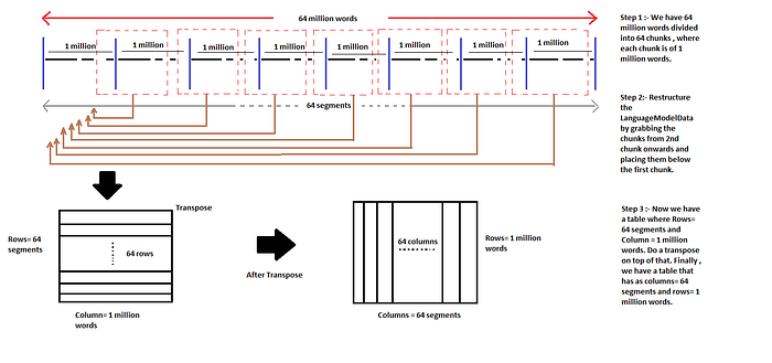
LanguageModelDatais a lot movie reviews. Then all of the movie reviews files gets concatenated together to form one big block of text. - Organizing the data. Lets talk about the concept of bptt, bs in detail. Suppose we have 64 million words or in other words say concatenated movie reviews. We split these words into batch size (bs=64). Then we organize the data as described in the image below.

Note :- In the table above , these 1 million words has been mapped into a integer IDs . So the final table consists of Integer Ids and not words.

bptt=70means to grab a 70 section long sequence and chuck it into a GPU . That’s defined as a batch . A batch in NLP is always of width bs (batch size=64) and each batch is a sequence of length upto bptt (bptt=70).- Our
LanguageModelDataobject will create batches with 64 columns (that's our batch size), and varying sequence lengths of around 80 tokens (that's ourbpttparameter - backprop through time). - What torchtext does is it randomly changes bptt number every time , so each epoch is getting slightly different bits of text. Its the same as shuffling images in computer vision. We can’t randomly shuffle the order of the words as it won’t make any sense . We need them in proper order , so that our model will learn the structure of English. Hence we instead move their breakpoints a little bit around 70 .
- Each batch also contains the exact same data as labels, but one word later in the text — since we’re trying to always predict the next word. The labels are flattened into a 1d array.
- To grab a batch of data, wrap it with iterator to turn it into a iterator. And call next on it to grab a batch of data. This is the form that Neural Network gets as an input . Lets have a look.
next(iter(md.trn_dl))
next(iter(md.trn_dl))[0].shape
- As we can see this batch has number of rows as bptt=67 and columns as batch size =64. This is our data.

- On a closer inspection to our model training dataset , we find that this dataset has been divided into two parts , one is our predictor part i.e the data we will use to do the prediction on (the part in red). And the other part is the target variable(the part in green).
- The target label shows exactly the same matrix but moved down by 1 as we are trying to predict the next word.
- Each batch also contains the exact same data as labels , but one word later in the text — since we are always trying to predict the next word. These labels are flattened into 1-d array.
Lets check other attribute that LanguageModelData provides us:-

len(md.trn_dl) # 4583 pieces we are going to go throughmd.nt # 37392 is the size of the vocab (Unique tokens).These unique words # have to appear more than 10 times or else they will be replaced by # unknowns(unk).len(md.trn_ds) # 1 because there is only 1 corpus from where we are # getting our words.len(md.trn_ds[0].text) # This corpus has 20.5 million words in it.
LETS START TRAINING OUR MODEL:-
- We have a number of parameters to set — we’ll learn more about these later, but you should find these values suitable for many problems.
em_sz = 200  # size of each embedding vector
nh = 500     # number of hidden activations per layer
nl = 3       # number of layers
md.nt (# 37392 )is the size of the vocab (Unique tokens). These unique words have to appear more than 10 times or else they will be replaced by unknowns(unk).- Each of these 37392 words , has an embedding vector of length =200 is associated with it . These are very high cardinal categorical variables.

- Since these words have a lot more nuance associated with them , so we have a such big embedding vector for each of them.
- Rule of thumb for embedding matrix size:
50< embedding size(em_sz) <600. - This is a
three layer neural network (nl)and thehidden layer (nh) has 500 activation. - Researchers have found that large amounts of momentum (which we’ll learn about later) don’t work well with these kinds of RNN models, so we create a version of the Adam optimizer with less momentum than it’s default of
0.9.
opt_fn = partial(optim.Adam, betas=(0.7, 0.99))- fastai uses a variant of the state of the art AWD LSTM Language Model developed by Stephen Merity. A key feature of this model is that it provides excellent regularization through Dropout. There is no simple way known (yet!) to find the best values of the dropout parameters below — you just have to experiment…
- However, the other parameters (
alpha,beta, andclip) shouldn't generally need tuning. - Creating the
learner.
learner = md.get_model(opt_fn, em_sz, nh, nl,
               dropouti=0.05, dropout=0.05, wdrop=0.1, dropoute=0.02, dropouth = 0.05, tmp_name=TMP_PATH, models_name=MODELS_PATH)
learner.reg_fn = partial(seq2seq_reg, alpha=2, beta=1)
# Reducing the overfitting
learner.clip=0.3- What
learner.clip=0.3does is it prevents overshooting while looking for local minima during gradient descent. Details don’t matter much for now.
Finally , lets Train our data by making use of fit command.
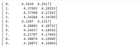
learner.fit(3e-3, 4, wds=1e-6, cycle_len=1, cycle_mult=2)learner.save_encoder('adam1_enc')learner.fit(3e-3, 4, wds=1e-6, cycle_len=10,
            cycle_save_name='adam3_10')learner.save_encoder('adam3_10_enc')learner.fit(3e-3, 1, wds=1e-6, cycle_len=20,
            cycle_save_name='adam3_20')learner.load_cycle('adam3_20',0)

For sentiment analysis , we need first section of the model i.e the encoder part , so lets save it :-
learner.save_encoder('adam3_20_enc')learner.load_encoder('adam3_20_enc')
Language modeling accuracy is generally measured using the metric perplexity, which is simply exp() of the loss function we used.
math.exp(4.165)
pickle.dump(TEXT, open(f'{PATH_WRITE}models/TEXT.pkl','wb'))
# Save the model
Before moving towards Sentiment analysis , lets check out how our model understands English structure as mentioned in IMDB dataset.
# We can play around with our language model a bit to check it seems to  # be working OK. First, let's create a short bit of text to 'prime' a set # of predictions. We'll use our torchtext field to numericalize it so we # can feed it to our language model.m=learner.model
ss=""". So, it wasn't quite was I was expecting, but I really liked it anyway! The best"""
s = [TEXT.preprocess(ss)]
t=TEXT.numericalize(s)
' '.join(s[0])# Set batch size to 1
m[0].bs=1
# Turn off dropout
m.eval()
# Reset hidden state
m.reset()
# Get predictions from model
res,*_ = m(t)
# Put the batch size back to what it was
m[0].bs=bs
#  Let's see what the top 10 predictions were for the next word after our # short text:
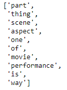
nexts = torch.topk(res[-1], 10)[1]
[TEXT.vocab.itos[o] for o in to_np(nexts)]

Lets see if our model is able to predict the next word by itself:-
res[-1].topk(3)[1]
# These three are the top three prediction for the next word in ascending order .
Lets generate next couple of words now:-
print(ss,"\n")
for i in range(50):
    n=res[-1].topk(2)[1]
    n = n[1] if n.data[0]==0 else n[0]
    print(TEXT.vocab.itos[n.data[0]], end=' ')
    res,*_ = m(n[0].unsqueeze(0))
print('...')
If I may direct your attention to the above snapshot, you can see that the model was able to correctly comprehend couple of words “part of the movie” after the given input . “So, it wasn’t quite was I was expecting, but I really liked it anyway! The best”. Post that , it wasn’t making sense . This is because , I didn’t train my model to the last epoch . After that , I trained my model until the very last epoch and got this as output.
". So, it wasn't quite was I was expecting, but I really liked it anyway! The best

film ever ! <eos> i saw this movie at the toronto international film festival . i was very impressed . i was very impressed with the acting . i was very impressed with the acting . i was surprised to see that the actors were not in the movie . ..."
SENTIMENT ANALYSIS
- If we are using some pre-trained model, we need the exact same vocab. The word “the” should still match to the #2 position, so that we can look up to the Embedding Vector corresponding to “the”. So we load our Field object , the thing in which we have the VOCAB in. To use a pre-trained model , we need to have the same VOCAB from the language model.We can use the following code if we need the same pre-trained model in a new seesion.
TEXT = pickle.load(open(f'{PATH}models/TEXT.pkl','rb'))- In the code below
sequential=Falsetells torchtext that a text field should be tokenized (in this case, we just want to store the ‘positive’ or ‘negative’ single label).
IMDB_LABEL = data.Field(sequential=False)
splits = torchtext.datasets.IMDB.splits(TEXT, IMDB_LABEL, 'data/')splitsis a torchtext method that creates train, test, and validation sets. The IMDB dataset is built into torchtext, so we can take advantage of that. Take a look atlang_model-arxiv.ipynbto see how to define your own fastai/torchtext datasets.- Earlier , we treated all the reviews as one big piece of text. But now each review is different as it has a positive or negative sentiment attached to it. So this time we will treat each review distinctly.
- Lets grab a particular example.
t = splits[0].examples[0]t.label, ' '.join(t.text[:16])

'pos'is the label which stands for positive andt.text[:16]is the actual movie review.- Once we have the
splitobject ready , convert the torchtext object into afastai objectformat so that we can train upon.
md2 = TextData.from_splits(PATH, splits, bs)- Now lets create the
Learner.
m3 = md2.get_model(opt_fn, 1500, bptt, emb_sz=em_sz, n_hid=nh, n_layers=nl,
           dropout=0.1, dropouti=0.4, wdrop=0.5, dropoute=0.05, dropouth=0.3)
m3.reg_fn = partial(seq2seq_reg, alpha=2, beta=1)
m3.load_encoder(f'adam3_10_enc')
Because we’re fine-tuning a pretrained model, we’ll use differential learning rates, and also increase the max gradient for clipping, to allow the SGDR to work better.
m3.clip=25.
lrs=np.array([1e-4,1e-4,1e-4,1e-3,1e-2])m3.freeze_to(-1)
m3.fit(lrs/2, 1, metrics=[accuracy])
m3.unfreeze()
m3.fit(lrs, 1, metrics=[accuracy], cycle_len=1)
m3.fit(lrs, 7, metrics=[accuracy], cycle_len=2, cycle_save_name='imdb2')
m3.load_cycle('imdb2', 4)
accuracy_np(*m3.predict_with_targs())
# 0.94310897435897434
That’s how we built a State of The Art Sentiment Analysis Classifier.
If you have reached until this i.e the end of this article . Great job .You deserve a clap. 👏 👏👏👏👏😃😃😃😃😃😃😃😃😃👏 👏👏👏👏👏
If you have any questions, feel free to reach out on the fast.ai forums or on Twitter:@ashiskumarpanda
P.S. -The code used here is present in my Github repository. This blog post will be updated and improved as I further continue with other lessons. For more interesting stuff , Feel free to checkout my Github account.
To make best out of this blog post Series , feel free to explore the first Part of this Series in the following order:-Dog Vs Cat Image Classification
- Dog Vs Cat Image Classification
- Dog Breed Image Classification
- Multi-label Image Classification
- Time Series Analysis using Neural Network
- NLP- Sentiment Analysis on IMDB Movie Dataset
- Basic of Movie Recommendation System
- Collaborative Filtering from Scratch
- Collaborative Filtering using Neural Network
- Writing Philosophy like Nietzsche
- Performance of Different Neural Network on Cifar-10 dataset
- ML Model to detect the biggest object in an image Part-1
- ML Model to detect the biggest object in an image Part-2
Edit 1:- TFW Jeremy Howard approves of your post . 💖💖 🙌🙌🙌 💖💖 .
