!!! WRITE PHILOSOPHY LIKE NIETZSCHE USING RNN !!!

The Concept of RNN is used for building this Language Model.

19 min readDec 2, 2018

To make best out of this blog post Series , feel free to explore the first Part of this Series in the following order:-

In Natural Language Programming , Language Modelling plays a crucial role .

But ,what is a Language Model ?
A language model is a model where given some characters, its able to predict what should be the next character. To do this , a language model should know how to read English , which means its should understand the structure of English Language. Once it understands the structure, it will be able to comprehend or predict the next character in a sentence.

This blog post deals with Language Modelling at a Character level. This model will be trained in such a way that it will be able to predict the next character , given a set of character as input . This blog post will use Pytorch to create a Language model from Scratch and slowly will increase the complexity of the model in steps , so as to come up with a really good model .

In this blog post , we will teach our model to write Philosophy like Nietzsche . For this purpose, we will be using RNN . Why RNN?

RNN is used for:-

Variable Length Sequence.
Long term dependency
Stateful Representation
Memory

Before getting started with RNN , lets understand Jeremy’s notation of Neural Network and then extend it to a RNN.

BASIC NEURAL NETWORK WITH SINGLE HIDDEN LAYER.

Every shape is a bunch of Activations. The arrow represents a layer operation which is a matrix product followed by a ReLU.
There is an input represented by a rectangle .The input is (batch_size ,#columns in our data) .
The input is followed by a Matrix product and a Relu . This give rise to Hidden Activations (the one represented by circle).
The hidden activations is followed by a Matrix product and a Softmax which gives rise to Output Activations (the one represented by triangle).

Next , lets check out Jeremy’s notation of RNN :-

RNN (RECURRENT NEURAL NETWORK)

PREDICTING THIRD CHARACTER USING PREVIOUS TWO CHARACTERS

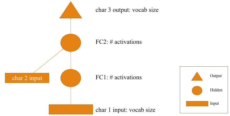
The first input here, is the first character in each mini batch. Each input character is represented by its embedding vector . This will be our input activations. Pass it via a fully connected layer (represented by an arrow) and the outcome is the hidden layer Activations represented by FC1.

NOTE:- An embedding vector is a random set of numbers which represents the particular character. It gets optimized during the training process.

Again , pass it via a 2nd fully connected layer and get some Activations represented by (FC2).
But this time the Activations are accompanied by the embedding vector of 2nd character. This embedding vector is followed by a matrix product(the arrow mark from char 2 input). So add up the input from character 2 Activations and the hidden layer activations. Both of these are supposed to be of same dimensions.
After adding both of them we get a FC2 Activations. Now put them through another matrix product followed by a softmax to get a predicted set of characters.
Here we are getting two characters as inputs and trying to predict the third character.

Lets get into coding part now .

LOAD ALL THE PACKAGES REQUIRED:-

%reload_ext autoreload
%autoreload 2
%matplotlib inlinefrom fastai.io import *
from fastai.conv_learner import *from fastai.column_data import *

DOWNLOAD NIETZSCHE CORPUS

Set the path and download the data. The corpus that will be used is a Nietzsche corpus.

PATH='/kaggle/working/nietzsche/'
get_data("https://s3.amazonaws.com/text-datasets/nietzsche.txt", f'{PATH}nietzsche.txt')
text = open(f'{PATH}nietzsche.txt').read()
print('corpus length:', len(text))

Corpus has 600893 characters in total (repetition inclusive). Check out a chunk of Nietzsche corpus text.

text[:400]

chars = sorted(list(set(text)))
# set() function takes distinct unique characters in the corpus.vocab_size = len(chars)+1
print('total chars:', vocab_size)

Total number of unique character in the whole of corpus is 85.

Sometimes it’s useful to have a zero value in the dataset, e.g. for padding

chars.insert(0, "\0")
''.join(chars[0:-6])
# Gives a glimpse of whats present in our dataset.

Map the characters into indices and indices to characters.

# Each character is mapped with an integer and vice-versa
char_indices = {c: i for i, c in enumerate(chars)}indices_char = {i: c for i, c in enumerate(chars)}

idx will be the data that will be used from now on — it simply converts all the characters to their index (based on the above mapping ).

idx = [char_indices[c] for c in text]idx[:10]

# Lets cross check by turning each number into character and join them    # together.
''.join([indices_char[i] for i in idx[:70]])

GETTING THE DATA INTO PROPER FORMAT:

The problem statement is to predict the fourth character given three character as input. To do that four lists are needed to be created. Three input and one target/labels.

First list starts from 0th position and will select every fourth item in the list .
Second list starts from 1st position and will select every fourth item in the list .
Third list starts from 2nd position and will select every fourth item in the list .
Fourth list starts from 3rd position and will select every fourth item in the list .
First , Second and Third list will be our input and Fourth list will be our output. So lets create some list and visualize it.

cs=3
c1_dat=[idx[i] for i in range(0,len(idx)-cs,cs)]
c2_dat=[idx[i+1] for i in range(0,len(idx)-cs,cs)]
c3_dat=[idx[i+2] for i in range(0,len(idx)-cs,cs)]
c4_dat=[idx[i+3] for i in range(0,len(idx)-cs,cs)]
# np.stack to pop them together################ INPUT #######################
x1=np.stack(c1_dat[:-2])
x2=np.stack(c2_dat[:-2])
x3=np.stack(c3_dat[:-2])
################################################################ LABELS ########################
x4=np.stack(c4_dat[:-2])
################################################print(x1)
print(x2)
print(x3)
print(x4)

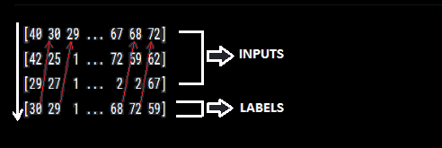
As seen in the output snapshot above , given 1st three letters , the model is suppose to predict every fourth letter . So our data has to be arranged in the same way . Traversing column wise is the actual way the letters has been arranged. x1,x2,x3 are the input and x4 is the output. It can be seen that after 40,42,29 comes 30 in the next column which is actually the label that our model is trying to learn, hence the label x4 value is 30 . Similarly for other columns.

It can also be seen in terms of characters. The first word is PREFACE , check out how its arranged.

print(''.join([indices_char[i] for i in x1[:70]][:3]))
print(''.join([indices_char[i] for i in x2[:70]][:3]))
print(''.join([indices_char[i] for i in x3[:70]][:3]))
print(''.join([indices_char[i] for i in x4[:70]][:3]))

After P,R,E (which has been arranged in a column )comes F (which is present in the next column ), hence our target variable is F. Similarly , after F,A,C comes E (which is present in the next column ) ,hence E is the target variable .

Our inputs are:-

x1 = np.stack(c1_dat)
x2 = np.stack(c2_dat)
x3 = np.stack(c3_dat)

Our output is :-

y = np.stack(c4_dat)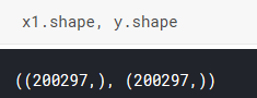

GET THE DATA READY AS PER FASTAI MODEL DATA FORMAT:

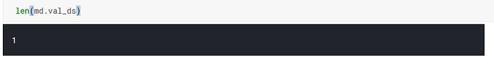
md = ColumnarModelData.from_arrays('.', [-1], np.stack([x1,x2,x3], axis=1), y, bs=512)

The above ColumnarModelData.from_arrays(...) helps in getting the data ready as per fastai format.
‘.’ represents the current PATH where the output model needs to be stored .
[-1] represents the validation data set. Its takes the last entry of np.stack([x1,x2,x3], axis=1),y as Validation dataset. Can be cross checked in the snapshot below.

np.stack([x1,x2,x3], axis=1) is our input or independent variable.
y is our target variable.
bs is our batch size.
CREATE AND TRAIN THE MODEL

The below image demonstrates the process of predicting the 4th character from first three characters.

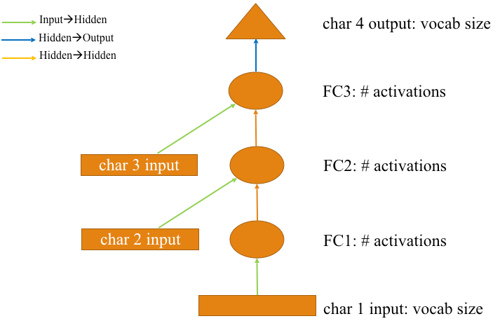
Green arrows represents the initial linear layer from input to hidden layer .

Orange Arrow represents the Hidden layer matrix from hidden to hidden layer.

Blue Arrow represents the Output Weight matrix from hidden to output layer .

Lets see the code that represents the above operation.

n_hidden = 256
n_fac = 42
vocab_size=85 # as we have total 85 distinct characters in this corpus.class Char3Model(nn.Module):
    def __init__(self, vocab_size, n_fac):
        super().__init__()
        self.e=nn.Embedding(vocab_size, n_fac)
        # (85,42)
        # The 'green arrow' from our diagram - the layer operation from input to hidden
        self.l_in = nn.Linear(n_fac, n_hidden)
         # (42,256)
        # The 'orange arrow' from our diagram - the layer operation from hidden to hidden
        self.l_hidden = nn.Linear(n_hidden, n_hidden)
         # (256,256)
        # The 'blue arrow' from our diagram - the layer operation from hidden to output
        self.l_out = nn.Linear(n_hidden, vocab_size)
        # (256,85)
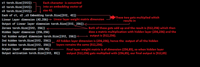
    def forward(self,c1,c2,c3):
#         print("c1",c1.size())
#         print("c2",c2.size())
#         print("c3",c3.size())
#         print("Each of c1, c2 ,c3 Embedding",self.e(c1).size())
#         print("Linear Layer dimension (42,256) ")
#         print("Output of Linear layer dimension",self.l_in(self.e(c1)).size())
        in1=F.relu(self.l_in(self.e(c1)))
        in2=F.relu(self.l_in(self.e(c2)))
        in3=F.relu(self.l_in(self.e(c3)))
        
        h=V(torch.zeros(in1.size()).cuda())
#         print("Zeroes",h.size())
#         print("Hidden layer dimension (256,256)")
        h=F.tanh(self.l_hidden(h+in1))
#         print("1st hidden output dimension",h.size())
        h=F.tanh(self.l_hidden(h+in2))
#         print("2nd hidden",h.size())
        h=F.tanh(self.l_hidden(h+in3))
#         print("3rd hidden",h.size())
#         print("Output layer  dimension (256,85)")
#         print("Output activation",self.l_out(h).size())
        return F.softmax(self.l_out(h))m = Char3Model(vocab_size, n_fac).cuda()it = iter(md.trn_dl)
*xs,yt = next(it)
t = m(*V(xs)) # Calls the forward function
t.size()

Create an object mby initializing a class with Char3Model(vocab_size, n_fac) .
.cuda() represents the operation to be performed on the GPU.
Whenever a class is initialized, the constructor def __init__(self, vocab_size, n_fac): , gets automatically invoked . Things with weights are created and initialized within the constructor.
super().__init__() :- This inherits all the special functions from nn.Module .
self.e=nn.Embedding(vocab_size, n_fac) creates the embedding matrix of size (vocab_size, n_fac) . In this case the size is (85,42).
self.l_in = nn.Linear(n_fac, n_hidden) represents the ‘green arrow’ from our diagram — the layer operation from input to hidden layer.In this case size is (42,256) .
self.l_hidden = nn.Linear(n_hidden, n_hidden) represents the ‘orange arrow’ from our diagram — the layer operation from hidden to hidden layer. In this case the size is (256,256) .
self.l_out = nn.Linear(n_hidden, vocab_size) represents the ‘blue arrow’ from our diagram — the layer operation from hidden to output layer. In this case the size is (256,85).
FLOW OF OPERATION

it = iter(md.trn_dl)
*xs,yt = next(it)
t = m(*V(xs)) # Calls the forward function
t.size()

md.trn_dl is a data loader having a mini-batch of data . To iterate over the data wrap it with a iter function .
next(it) grabs the next mini-batch of data , each time its executed .
m(*V(xs)) In Pytorch we have to convert our tensors into Variable . It helps in backpropagating through the tensors. Hence we use V(xs) . m(*V(xs)) calls the forward function which returns the output as shown in the above snapshot , which is of size [512,85] . Since the dataset has 85 unique characters , it returns the probability value for each of those character in the minibatch data.

Let’s do a deep dive into the forward function .

The length of input data (xs )is 3.

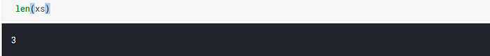
The forward function expects three characters (c1, c2, c3) and xs is of length 3 .
Each of the character is passed through embedding layer , then linear layer and finally through ReLU. This is done using the below command :

in1 = F.relu(self.l_in(self.e(c1)))
in2 = F.relu(self.l_in(self.e(c2)))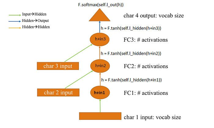
in3 = F.relu(self.l_in(self.e(c3)))

The below commands can be described using the RNN diagram as shown below :

h = V(torch.zeros(in1.size()).cuda())
h = F.tanh(self.l_hidden(h+in1))
h = F.tanh(self.l_hidden(h+in2))
h = F.tanh(self.l_hidden(h+in3))
return F.softmax(self.l_out(h))

The flow operation can be represented by this flowchart image and the below output image.

opt = optim.Adam(m.parameters(), 1e-2)

The optimizer that will be used here is Adam Optimizer .
m.parameters() are the parameters of the models that are needed to be optimized.
The learning rate to be used is 1e-2 .

TRAINING THE MODEL:

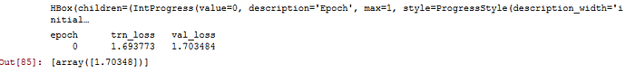
fit(m, md, 1, opt, F.nll_loss)

fit (...) helps in training the data.
md : Model data as per fastai format.
m : The class Char3Model , declared above helps in initializing the parameters and steps mentioned in the forward function of the class, decides the functions performed by the RNN, which helps in training the data.
1 : 1 epoch over the dataset.
opt :optimizers to be used.
F.nll_loss : Loss function that’s needed to be minimized to get the optimum value for parameters.
The output shows the loss after 1 epoch .

Lets change our learning rate to see if the loss function value could be minimized.

set_lrs(opt, 0.001)
fit(m, md, 1, opt, F.nll_loss)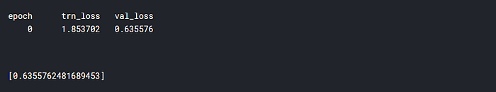

DO THE PREDICTION:

def get_next(inp):
    idxs = T(np.array([char_indices[c] for c in inp]))
    p = m(*VV(idxs))
    print(p.size()) #Spits out the 85 probabilities
    i = np.argmax(to_np(p))
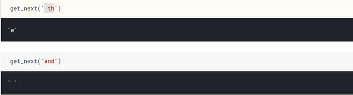
    return chars[i]get_next(' th')

The 3 characters “ th“ is passed as an input (inp).
Those three characters are turned into mapped integers . And are converted into Tensor.
p = m(*VV(idxs)):- Turn those into Variables using *VV(idxs) and pass it into the model.
p spits out 85 probabilities number for 85 vocab present in our corpus.
Choose the highest probability value using np.argmax(to_np(p)) .This helps in grabbing the character which has the highest probability of coming up next.

When ‘ th’ is passed as input , it predicts e .Kind of makes sense. It means it has gone through the corpus and understood the structure of English language.

OPTIMIZED VERSION OF RNN

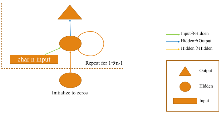
The above RNN flow chart diagram could be reduced to a simplified version like this image below . The dotted square box denotes the part that will be included in the for loop and it will replace the repetitive hidden layer .

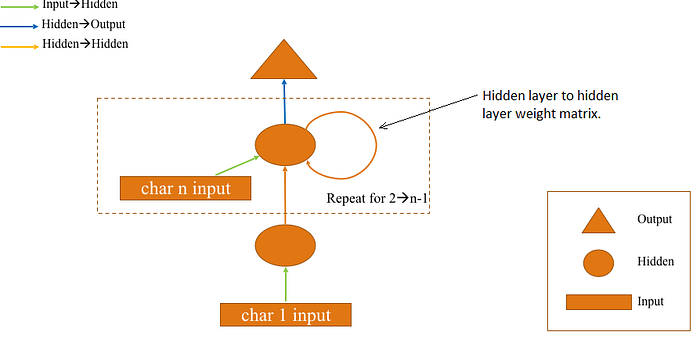
Since the first character has been passed as an input separately , hence the repetition occurs within the for loop for 2nd character to n-1 character .

Let’s now create a more optimized model where given eight characters , our model will predict the 9th character.

Note:- Number of character that will be given as input will be the same as number of hidden layer. So in this case , our model has 8 hidden layer.

GIVEN EIGHT CHARACTERS PREDICT THE 9TH CHARACTER

cs=8
c_in_dat = [[idx[i+j] for i in range(cs)] for j in range(len(idx)-cs)]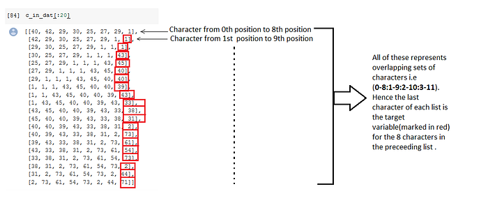

c_out_dat = [idx[j+cs] for j in range(len(idx)-cs)]
c_out_dat[:20]

c_out_dat is the label . And on the basis of this , it can be cross verified with the red ones in the above image .

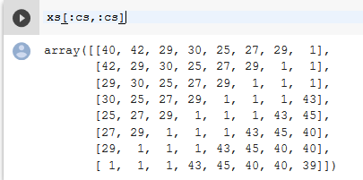
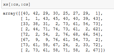
xs = np.stack(c_in_dat, axis=0) # Stack all your inputs
xs.shape# (600885, 8)

Our input data:-

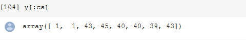
y = np.stack(c_out_dat) #Stack all your outputs.
y.shape# (600885,)

Our output/Target data:-

CREATE AND TRAIN A MODEL:

val_idx= get_cv_idxs(len(idx)-cs-1)
md = ColumnarModelData.from_arrays('.', val_idx, xs, y, bs=512)class CharLoopModel(nn.Module):
    # This is an RNN!
    def __init__(self, vocab_size, n_fac):
        super().__init__()
        self.e = nn.Embedding(vocab_size, n_fac)
        self.l_in = nn.Linear(n_fac, n_hidden)
        self.l_hidden = nn.Linear(n_hidden, n_hidden)
        self.l_out = nn.Linear(n_hidden, vocab_size)
        
    def forward(self, *cs):
        bs = cs[0].size(0)
        h = V(torch.zeros(bs, n_hidden).cuda())
        for c in cs:
            inp = F.relu(self.l_in(self.e(c))) 
            h = F.tanh(self.l_hidden(h+inp))
        return F.log_softmax(self.l_out(h), dim=-1)

In the above code , a RNN is created , the only difference in this code and the previous code is that , this code is more optimized i.e instead of writing commands for calculating the input activations and hidden layer activations for all the eight characters separately , just wrap it up in a for loop.
Inside the for loop , all the characters are called upon one by one and using this command inp = F.relu(self.l_in(self.e(c))) , it is being :-

Passed through the embedding vector .

2. Then through the input Linear layer .

3. And then through the ReLU activation function. This gives us inp .

In the next step within for loop i.e h = F.tanh(self.l_hidden(h+inp)) :-
The hidden layer activations and the input activations are added up.
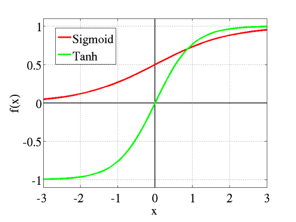
Pass it through a hidden layer and then through a tanh activation.
Tanh activation is used in hidden to hidden state transition as it stops from blowing up the values . In deep Layered Neural Network , there is a great probability that the matrix multiplication output values would be too high .Hence tanh summarizes it between -1 to 1 . Check out tanh activation graph.
Repeat the same old steps as shown below

# Create the model data as per fastai format.
md = ColumnarModelData.from_arrays('.', val_idx, xs, y, bs=512)# Initialize the parameters
m=CharLoopModel(vocab_size,n_fac).cuda()# Choose an optimizer to optimize the parameters.
opt=optim.Adam(m.parameters(),1e-2)# Train the model by passing appropriate parameters
fit(m, md, 1, opt, F.nll_loss)

set_lrs(opt,0.001)
fit(m, md, 1, opt, F.nll_loss)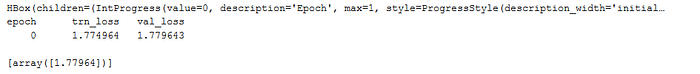

As seen, the loss value has drastically reduced after changing the learning rate. Lets pass some value as input to see how our model is performing.
After passing 8 characters , its able to predict the last letter of the word woman .

FURTHER IMPROVING THE MODEL

Until now, the input state and the hidden state activations were added .
The input state activations and the hidden state activations are qualitatively two different kind of things. Input state activations is the encoding of the character and hidden state represent the encoding of series of characters so far .
Adding leads to loss of information , so just concatenate instead of adding . By concatenating , different kind of information can be combined.

CONCATENATING INSTEAD OF ADDING:

class CharLoopConcatModel(nn.Module):
    def __init__(self, vocab_size, n_fac):
        super().__init__()
        self.e = nn.Embedding(vocab_size, n_fac)
        self.l_in = nn.Linear(n_fac+n_hidden, n_hidden)
        self.l_hidden = nn.Linear(n_hidden, n_hidden)
        self.l_out = nn.Linear(n_hidden, vocab_size)
        
    def forward(self, *cs):
        bs = cs[0].size(0)
        h = V(torch.zeros(bs, n_hidden).cuda())
        for c in cs:
            inp = torch.cat((h, self.e(c)), 1)
            inp = F.relu(self.l_in(inp))
            h = F.tanh(self.l_hidden(inp))
        
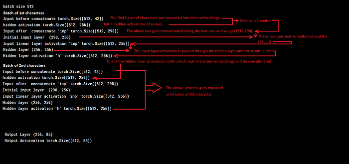
        return F.log_softmax(self.l_out(h), dim=-1)

The code is almost exactly same as the previous one but we have got two changes.
self.l_in = nn.Linear(n_fac+n_hidden, n_hidden) . In this line , the dimension of input linear layer is changed .
Within the for loop ,inp = torch.cat((h, self.e(c)), 1) , instead of adding up , concatenation along the last axis takes place . The above code can be explained using the below snapshot.

Lets train the model using the same code snippets we used before:-

m = CharLoopConcatModel(vocab_size, n_fac).cuda()
opt = optim.Adam(m.parameters(), 1e-3)it = iter(md.trn_dl)
*xs,yt = next(it)
t = m(*V(xs))fit(m, md, 1, opt, F.nll_loss)
set_lrs(opt, 1e-4)
fit(m, md, 1, opt, F.nll_loss)

The loss has been reduced significantly in concatenating model as compared to adding up model. Hence the model is performing much better.
Lets do some validation , by predicting the 9th character on a set of 8 characters.

def get_next(inp):
    idxs = T(np.array([char_indices[c] for c in inp]))
    p = m(*VV(idxs))
    i = np.argmax(to_np(p))
    return chars[i]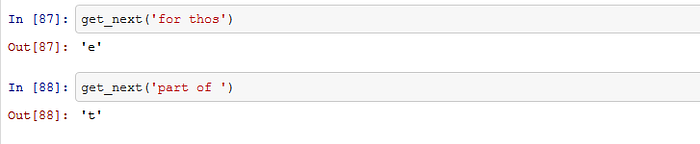

Now , let’s use PyTorch’s in-build functionalities for RNN.

RNN IN PYTORCH

Let’s get the code more optimized using the RNN function in PyTorch module .The advantages of using RNN function in PyTorch module is:-

It will handle the creation of linear layers automatically.
Replace the for loop that is within the forward function with nn.RNN() functionalities provided by PyTorch.

n_hidden = 256
n_fac = 42class CharRnn(nn.Module):
    def __init__(self, vocab_size, n_fac):
        super().__init__()
        self.e = nn.Embedding(vocab_size, n_fac)
        self.rnn = nn.RNN(n_fac, n_hidden)
        self.l_out = nn.Linear(n_hidden, vocab_size)
        
    def forward(self, *cs):
        bs = cs[0].size(0)
        h = V(torch.zeros(1, bs, n_hidden))
        inp = self.e(torch.stack(cs))
        outp,h = self.rnn(inp, h)
        
        return F.log_softmax(self.l_out(outp[-1]), dim=-1)

As said earlier , the above code handles the creation of linear layers automatically . This is achieved by using this line of code:- self.rnn = nn.RNN(n_fac, n_hidden) .
In the forward function , initialize the hidden activation with bunch of zeroes. Just like in earlier case this is the starting point for the for loop .
Using the inp = self.e(torch.stack(cs)) , get the embeddings for the characters.
This code outp,h = self.rnn(inp, h) performs exactly what happened within the for loop in case of CharLoopModel class previously. Pass the input and initial hidden state parameters and get the output and the final hidden state value.
In outp,h ,the outp keeps a track of all the hidden layer activations at the intermediate hidden layer , and the h has the final hidden layer activation.
Using this command F.log_softmax(self.l_out(outp[-1]), dim=-1) , get the final hidden layer activation self.l_out(outp[-1]) and pass it through the output activation i.e F.log_softmax.

m = CharRnn(vocab_size, n_fac).cuda()
opt = optim.Adam(m.parameters(), 1e-3)it = iter(md.trn_dl)
*xs,yt = next(it)t = m(*V(xs)); t.size()

fit(m, md, 4, opt, F.nll_loss)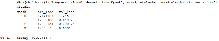

Change the learning rate and train it for a couple of epochs.

set_lrs(opt, 1e-4)
fit(m, md, 2, opt, F.nll_loss)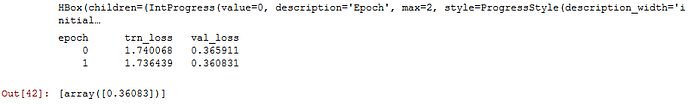

DO THE PREDICTION

def get_next(inp):
    idxs = T(np.array([char_indices[c] for c in inp]))
    p = m(*VV(idxs))
    i = np.argmax(to_np(p))
    return chars[i]get_next('for thos')

def get_next_n(inp, n):
    res = inp
#     
    for i in range(n):
        c = get_next(inp)
#         print(c)
        res += c
        inp = inp[1:]+c
#         print(inp)
    return resget_next_n('for thos', 50)

BEST EFFICIENT RNN MODEL (MULTI-OUTPUT MODEL) :-

To further optimize the model for better performance , use Multi-Output Model.

Earlier our way of dealing with data was highly inefficient . Why ?

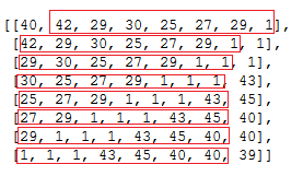
Its clear from the snapshot below that the red covered areas are the letters for which the embedding were being calculated . As seen there are redundancies involved i.e the same letters embeddings are being re-calculated each and every time. 7 out of 8 letter’s embedding are getting overlapped.

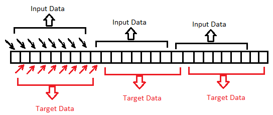
This is how a multi-model output looks like:-

As seen from the diagram above , everything inside the rectangular box is within for loop i.e for each input the model spits out an output. In multi-model approach , the model takes non-overlapping sets of character . Hence the redundancies is reduced. Lets get the input data and target variable ready for multi-output model.

cs=8
# That's our input saved as  c_in_dat.
c_in_dat = [[idx[i+j] for i in range(cs)] for j in range(0, len(idx)-cs-1, cs)]# For output/labels , create the same thing , offset by 1 saved as c_out_dat.
c_out_dat = [[idx[i+j] for i in range(cs)] for j in range(1, len(idx)-cs, cs)]xs = np.stack(c_in_dat)
xs.shape(75111, 8)ys = np.stack(c_out_dat)
ys.shape(75111, 8)

The input now is :-

The target variable now is:-

As seen from the above snapshot , there are no overlap . This can be represented diagrammatically :-

For every input , predict the next letter . Hence for every letter in our input data set , the succeeding letter is present as the target variable. And in this way , the overlapping has been prevented in the input dataset .For Each character that is being passed as an input to the model, there should be an output present. That’s what being represented in the Multi-Output model flowchart as shown above.

CREATE AND TRAIN MULTI-OUTPUT MODEL :-

val_idx = get_cv_idxs(len(xs)-cs-1)
md = ColumnarModelData.from_arrays('.', val_idx, xs, ys, bs=512)class CharSeqRnn(nn.Module):
    def __init__(self, vocab_size, n_fac):
        super().__init__()
        self.e = nn.Embedding(vocab_size, n_fac)
        self.rnn = nn.RNN(n_fac, n_hidden)
        self.l_out = nn.Linear(n_hidden, vocab_size)        
    def forward(self, *cs):
        bs = cs[0].size(0)
        h = V(torch.zeros(1, bs, n_hidden))
        inp = self.e(torch.stack(cs))
        outp,h = self.rnn(inp, h)
        return F.log_softmax(self.l_out(outp))

Its exactly the same as previous code , except some changes in the bold lettered code. The coding details of the multi-output model will be discussed in the next blog post . As we saw in this code , RNN isn’t good in predicting long sentence , hence we will look into other special type of RNNs like GRU and LSTM which will serve the purpose. The github repo at the end of this blogpost covers both RNN and LSTM and we can see how the LSTMs are predicting the next couple of words in Nietzsche style .

If you have reached until this i.e the end of this article . Great job .

YOU PEOPLE ROCK 👏 👏👏👏👏😃😃😃😃😃😃😃😃😃👏 👏👏👏👏👏

If you have any questions, feel free to reach out on the fast.ai forums or on Twitter:@ashiskumarpanda

P.S. -The code used here is present in my Github repository. This blog post will be updated and improved as I further continue with other lessons. For more interesting stuff , Feel free to checkout my Github account.

To make best out of this blog post Series , feel free to explore the first Part of this Series in the following order:-Dog Vs Cat Image Classification

Edit 1:- TFW Jeremy Howard approves of your post . 💖💖 🙌🙌🙌 💖💖 .

!!! WRITE PHILOSOPHY LIKE NIETZSCHE USING RNN !!!

The Concept of RNN is used for building this Language Model.

Written by Ashis Kumar Panda